  company avg_salary
1       A         95
2       B        155
3       C        109
4       D        166
5       E        173
6 F 65Showing Top & Bottom values in one clear visualization
A simple pattern to compare extremes of a distribution
data-wrangling
functions
R-Hacks N.4
This hack is based on my analysis on Kaggle analysis linked as follows (please see Chapter 4.3):
🔗 https://www.kaggle.com/code/lcolon/exploring-2024-software-engineer-salaries
When exploring a distribution, a very common question is:
Who are the top performers, and who are at the bottom?
Showing only the Top values might hid some context, while showing two separate charts can make comparison harder.
This R-Hack shows a simple and reusable pattern to display Top and Bottom values together in a single, clean visualization, as the one showed below:
Step 0 – Create an example dataset
Let’s start from a small, simulated dataset representing average salaries for different companies:
Step 1 – Build Top & Bottom datasets in a single pipeline
In this step, we extract both the Top 10 and Bottom 10 values using a single, readable pipeline.
The idea is simple. Starting from the same dataset:
select the Top 10 by applying
slice_max(), which returns all observations within the top 10 ranking positions, including any tiesselect the Bottom 10 by applying
slice_min(), returning all observations within the lowest 10 ranking positions, again including tiesassign a clear group label to each subset
combine the two subsets into a single dataframe for visualization and further analysis
  company avg_salary  group
1       X        179 Top 10
2       K        175 Top 10
3       T        175 Top 10
4       E        173 Top 10
5       P        168 Top 10
6       H        167 Top 10
Step 2 - Plot the data
In this step, starting from the dataframe created in the previous step, we build a simple visualization with ggplot:
plot_base <- ggplot(plot_df,
                    aes(x = reorder(company, -avg_salary), y = avg_salary)) +
  geom_col(fill = "steelblue") +
  geom_text(aes(label = avg_salary), vjust = -0.4, size = 4) +
  facet_wrap(~ fct_rev(group), scales = "free_x") +
  labs(
    title = "Top and Bottom Companies by Average Salary",
    subtitle = "Simulated data example\n\n",
    y = "Average yearly salary",
    x = NULL
  ) +
  theme_minimal() +
  theme(
    panel.grid = element_blank(),
    axis.text.x = element_text(size = 10),
    axis.text.y = element_blank()
  )

plot_base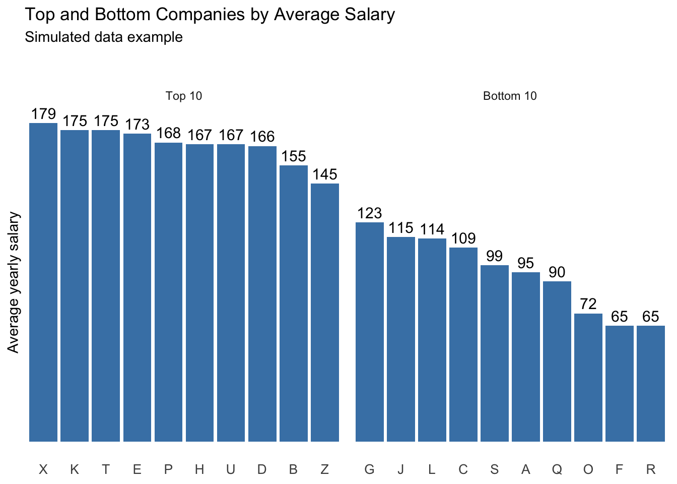
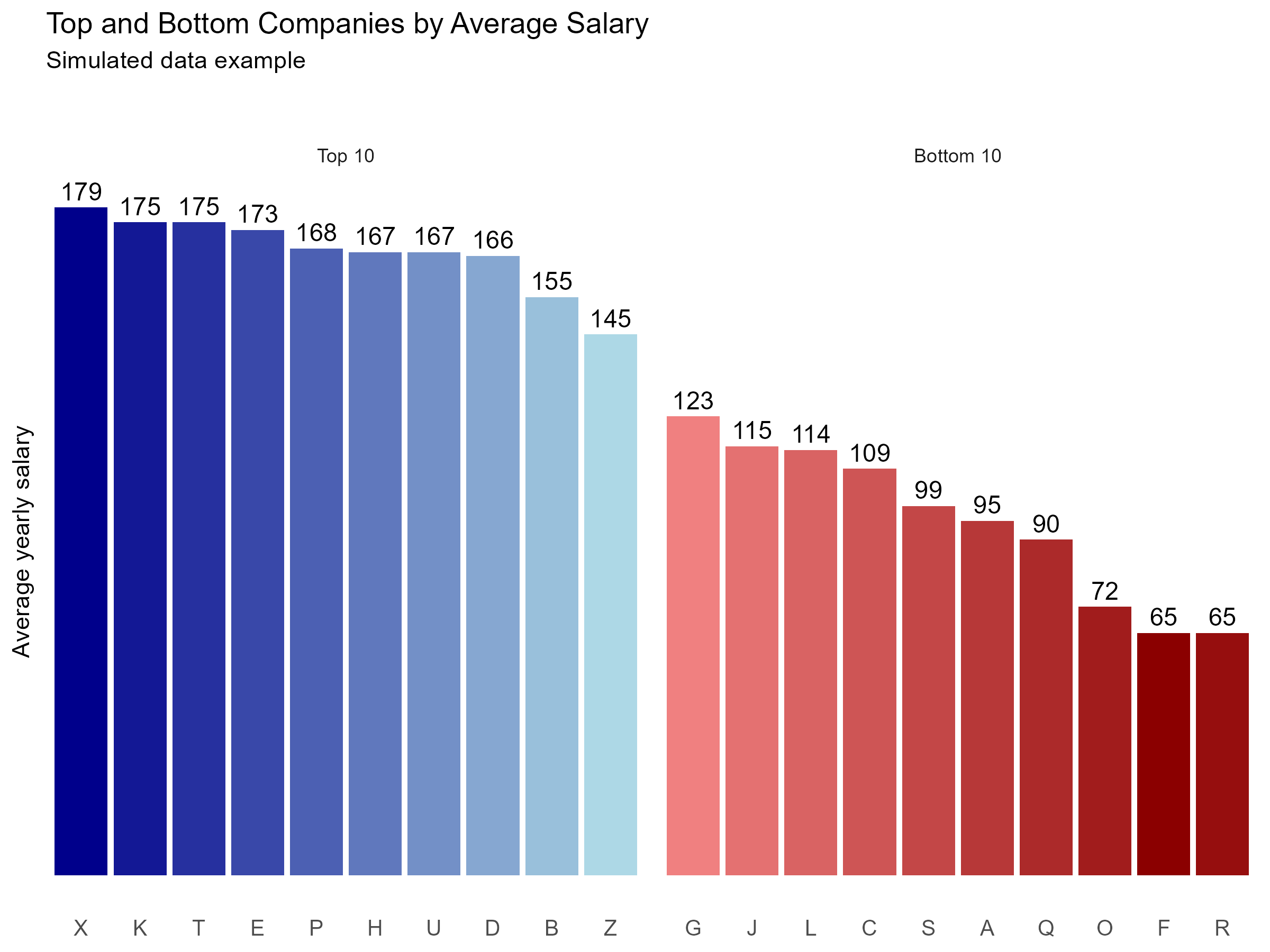
Step 3 - Generate gradient color palettes
Now that the base chart is working, we can make it more informative by adding two gradient color palettes:
- one gradient for the Top group (blue shades)
- one gradient for the Bottom group (red shades)
Instead of assigning a single color per group, we assign a slightly different shade to each bar. This creates a clean gradient effect while keeping the plot readable — even when ties produce more than 10 observations per group.
To do this, we:
- generate a group-specific palette with
colorRampPalette(), sized to the number of rows in each group (so it adapts if ties expand the selection) - group the data by
group(Top vs Bottom) - assign colors row by row using
row_number() - store the result in a new column called
color
plot_df <- plot_df %>%
  group_by(group) %>%
  mutate(
    color = if_else(
      group == "Top 10",
      colorRampPalette(c("darkblue", "lightblue"))(n())[row_number()],
      colorRampPalette(c("darkred", "lightcoral"))(n())[row_number()]
    )
  ) %>%
  ungroup()

head(plot_df)
# A tibble: 6 × 4
company avg_salary group color
<chr> <dbl> <chr> <chr>
1 X 179 Top 10 #00008B
2 K 175 Top 10 #131895
3 T 175 Top 10 #26309F
4 E 173 Top 10 #3948A9
5 P 168 Top 10 #4C60B3
6 H 167 Top 10 #6078BDStep 4 - Style the chart using the new colors
At this point, we don’t want to rewrite the entire ggplot call. Instead, we:
reuse the base chart (
plot_base)replace its dataset with the updated
plot_df(the one that now includes color) using the%+%operatoradd a new
geom_col()that maps fill to the color columnuse
scale_fill_identity()soggplotuses the colors as they are listed in thecolorcolumn
plot_styled <- (plot_base %+% plot_df) +
  geom_col(aes(fill = color)) +
  scale_fill_identity()

plot_styled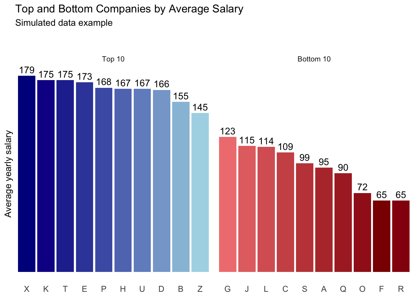
In short
Extract Top 10 and Bottom 10 values from the same dataset using
slice_max()andslice_min(), including tiesCombine the two subsets into a single dataframe for a compact overview of the distribution extremes
Build a clean base plot to validate structure and layout
Enhance the visualization by applying gradient colors to distinguish Top and Bottom groups
Tip
If you want to stay up to date with the latest events from the Rome R Users Group, click here:
👉 https://www.meetup.com/rome-r-users-group/
And if you are curious, the full Kaggle notebook used for this tip is available here:
🔗 https://www.kaggle.com/code/lcolon/exploring-2024-software-engineer-salaries