R Hack – Getting started with maps in R using GeoJSON and library sf
A simple workflow to load and plot maps in R
This hack is based on my Cyclistic analysis on Kaggle (see Chapter 8.12.4):
🔗 https://www.kaggle.com/code/lcolon/cyclistic-2023-google-da-capstone-project-r
Working with maps in R is easier than it seems.
If you want to visualize points, regions, or spatial patterns, the combination of GeoJSON files and the sf package gives you a simple and modern workflow.
In this hack, we’ll load a real city map (Chicago) directly from a URL, plot it with geom_sf(), and overlay simple point data.
Step 0 – What is a GeoJSON file?
A GeoJSON file is a JSON text file that stores geographic shapes (points, lines, polygons), together with their attributes (names, boundaries, codes, etc.).
It is one of the most common formats for open geographic data because it is lightweight, human-readable, and web-friendly.
You can often find GeoJSON files on:
- city open data portals (City of Chicago, NYC Open Data, etc.)
- national and international platforms (e.g., data.gov)
- GitHub repositories
- many public mapping resources
Step 1 – Load the required packages
Step 2 – Read a GeoJSON map with sf::st_read()
In this hack, we use a GeoJSON of Chicago community areas, provided by the City of Chicago Open Data Portal.
⚠️ Before using any online map or dataset, always remember to check the terms of use of the source.
You can read a GeoJSON directly from a URL, without downloading anything manually:
Simple feature collection with 6 features and 4 fields
Geometry type: MULTIPOLYGON
Dimension:     XY
Bounding box:  xmin: -87.74141 ymin: 41.80189 xmax: -87.60641 ymax: 41.93272
Geodetic CRS:  WGS 84
           pri_neigh          sec_neigh    shape_area    shape_len
1    Grand Boulevard        BRONZEVILLE 48492503.1554 28196.837157
2       Printers Row       PRINTERS ROW 2162137.97139  6864.247156
3      United Center      UNITED CENTER 32520512.7053 23101.363745
4 Sheffield & DePaul SHEFFIELD & DEPAUL 10482592.2987 13227.049745
5      Humboldt Park      HUMBOLDT PARK 125010425.593 46126.751351
6      Garfield Park      GARFIELD PARK 89976069.5947  44460.91922
                        geometry
1 MULTIPOLYGON (((-87.60671 4...
2 MULTIPOLYGON (((-87.62761 4...
3 MULTIPOLYGON (((-87.66707 4...
4 MULTIPOLYGON (((-87.65833 4...
5 MULTIPOLYGON (((-87.7406 41...
6 MULTIPOLYGON (((-87.6954 41...
What you get:
-
map_of_chicagois an sf object -essentially a data frame with a special geometry column where each row is a polygon that represents one community area
Step 3 – Plot a basic map with geom_sf()
Once the GeoJSON file has been loaded into an sf object, you can visualize it with geom_sf().
geom_sf() is the ggplot2 layer designed specifically for spatial data: it knows how to read the geometry column of an sf object and automatically draw points, lines, or polygons depending on what the data contains. In our case, it will draw the polygons of Chicago’s community areas.
ggplot() +
  geom_sf(data = map_of_chicago,
          fill = "#f1f0f0", color = "grey50") +
  labs(title = "Chicago community areas",
       subtitle = "GeoJSON map loaded with sf::st_read()") +
  theme_void()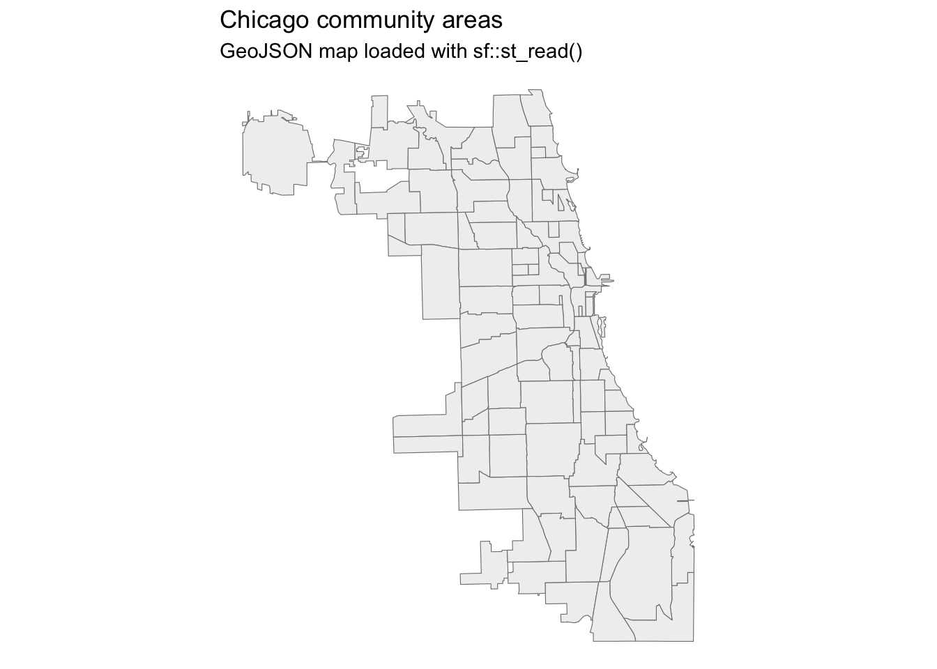
Step 4 – Add your own data on top of the map
If you have a dataset with latitude/longitude, you can overlay it on the map.
For example, let’s create a small dummy dataset of bike sharing station locations:
stations <- data.frame(
  start_lng = c(
    -87.6278, -87.6560, -87.6705, -87.6045, -87.5950,
    -87.6850, -87.6515, -87.7080, -87.6405, -87.5600),
  start_lat = c(
    41.8925, 41.9000, 41.9120, 41.8560, 41.7920,
    41.9220, 41.9250, 41.8810, 41.9410, 41.7600)
  )

stations
start_lng start_lat
1 -87.6278 41.8925
2 -87.6560 41.9000
3 -87.6705 41.9120
4 -87.6045 41.8560
5 -87.5950 41.7920
6 -87.6850 41.9220
7 -87.6515 41.9250
8 -87.7080 41.8810
9 -87.6405 41.9410
10 -87.5600 41.7600Now we can plot the base map plus the stations:
ggplot() +
  geom_sf(data = map_of_chicago,
          fill = "#f1f0f0", color = "grey70") +
  geom_point(data = stations,
             aes(x = start_lng, y = start_lat),
             color = "red",
             size = 3) +
  labs(title = "Bike stations on top of a GeoJSON map of Chicago",
       subtitle = "Base map: Chicago community areas (GeoJSON + sf)") +
  theme_void()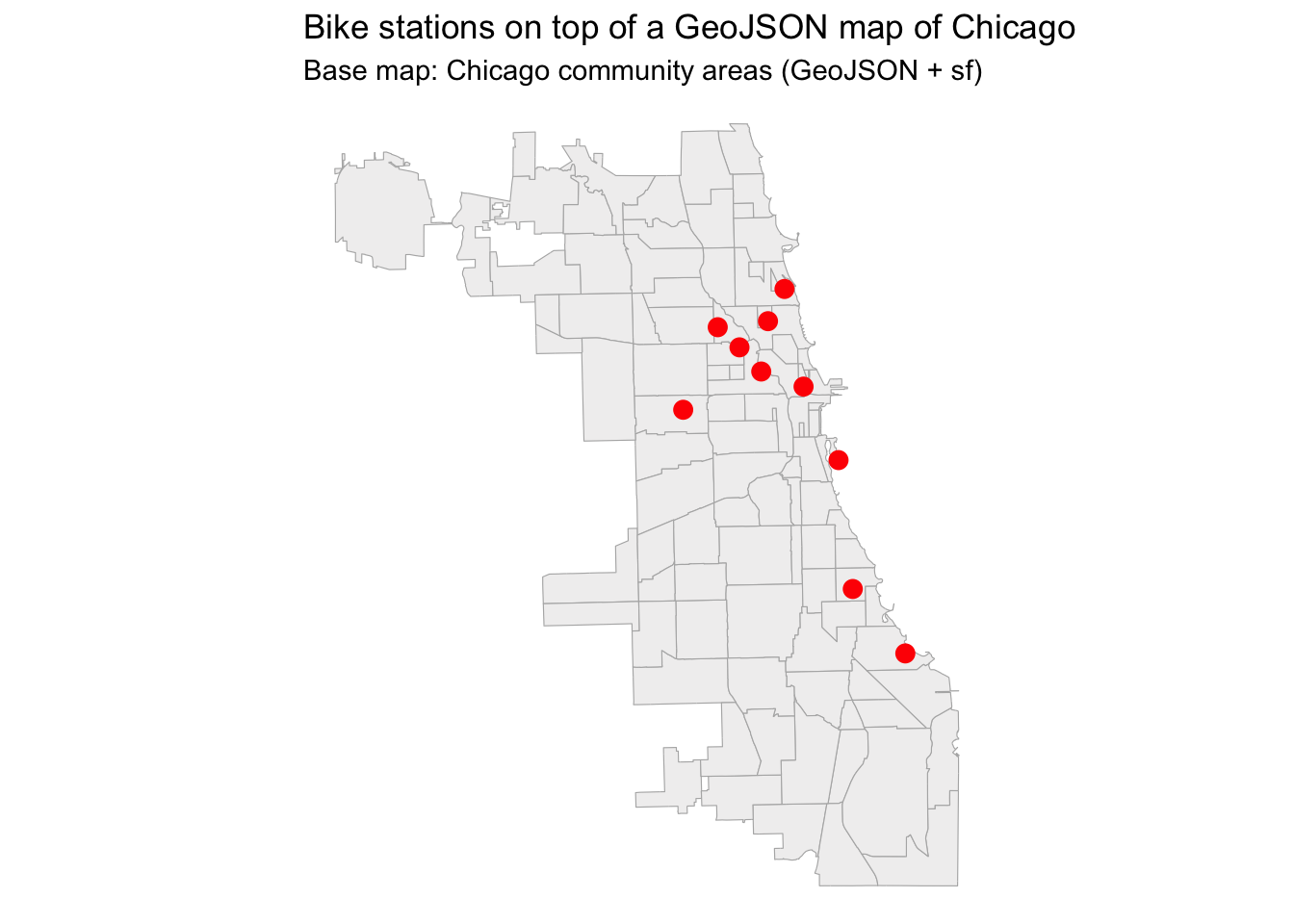
To Recap
GeoJSON = JSON file with geometry + attributes
Load it directly from a URL with
sf::st_read()Plot it with
geom_sf()Add your own points using regular ggplot layers
This workflow is simple, beginner-friendly, and requires no GIS tools
Thanks for reading!
If you want to stay up to date with the latest events from the Rome R Users Group, click here:
👉 https://www.meetup.com/rome-r-users-group/
And if you are curious, the full Kaggle notebook used for this tip is available here:
🔗 https://www.kaggle.com/code/lcolon/cyclistic-2023-google-da-capstone-project-r